Flow Visualization · CFD Validation
A fuel that mixes
without grids
- Helical cruciform fuel (HCF)
- Three-dimensional velocity fields by magnetic resonance velocimetry (MRV)
- CFD validation
Twist a fuel rod and the coolant mixes itself. What actually happens inside, though, nobody had seen. Using the same kind of MRI scanner found in a hospital, we measured the whole three-dimensional velocity field and looked in for the first time.
- Hyun Gi Moon
- Hangfei Dong
- S. Oh
 Min Seop Song
- S. Song
01 — Why this fuel
Running longermeans cooling better
One way to improve SMR economics is to run longer on a single fuel load. Higher-assay enriched uranium (HALEU) can stretch the cycle and shrink the core. But the same volume then carries more power, so unless the heat comes out faster, the safety margin shrinks with it.
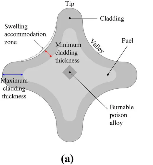
Metallic fuel is drawing renewed attention for exactly this reason: it conducts heat well and, just as importantly, it can be formed into whatever shape you want. Helical cruciform fuel (HCF) uses that freedom. Take a four-petal cruciform cross-section, twist it slowly along the axis, and the coolant swirls down the valleys and mixes itself.
Earlier work found that this shape substantially increases the heated surface area and, more importantly, can do away with spacer grids. Grids hold the rods in place but cost pressure drop. Mixing without them means pulling out more heat for less pumping power.
Heated surface area gain for an optimized geometry — BWR +29%, PWR +40% (Conboy et al.)
02 — The geometry
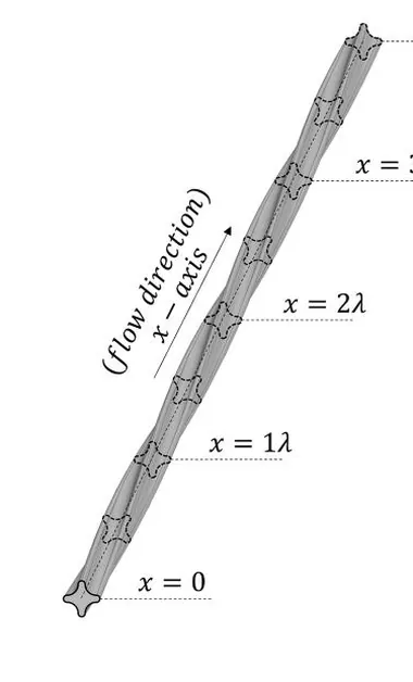
A four-petal section turning along the axis
The cross-section is a cruciform with four petals. Their tips almost touch the neighbouring rods, so the rods support one another. As the section turns along the axis, the open space between the rods, the subchannel, turns with it.
Drag the handle
- Twist pitch λ
- 17.1cm
- Over one pitch the cross-section turns 90° and returns to the same shape
- Axial distance
- 4.3cm
- Subchannel
- The open space enclosed by four rods, the path the coolant takes
03 — The problem
There was no wayto see inside
Putting this geometry into a design requires validated correlations, and building correlations requires a measured velocity field. Yet for HCF subchannels no PIV-level three-dimensional velocity dataset had ever been published.
Optical measurement is the obstacle. The gaps between rods are narrow and the surfaces are curved everywhere, so light bends at every boundary. Insert a probe and you change the very flow you came to measure. Earlier studies were limited to quantities measurable from outside, such as pressure drop and outlet concentration, and on the simulation side, RANS could not even reproduce the pressure drop.
04 — The method
Measuring with magnetism instead of light
Magnetic resonance velocimetry (MRV) works on the same principle as a hospital MRI. Apply a gradient to the magnetic field and fluid that travels farther in the same time picks up a larger shift in the phase of its signal. Read that shift and you have the velocity. Since no light is involved, neither opacity nor complex geometry gets in the way.
Encoding velocity separately along three directions yields the full three-component field throughout the volume. The trade is time: each acquisition is slow, so what you get is the time-averaged field rather than its instantaneous variation.
05 — The test section
3D-printed, then placed in the scanner
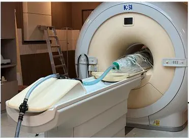
The 3 × 3 bundle was printed by stereolithography and five segments were joined to span five twist pitches. Everything entering the magnet had to be non-magnetic, down to polycarbonate fasteners. The pump and flowmeter sat in a separate control room with an observation window; only the hoses crossed into the magnet room.
We also checked the printed surface. Its roughness Reynolds number came out at 2.36, within the hydraulically smooth regime (below 5), so the print finish is unlikely to have altered the secondary-flow structures we measured.

- Array
- 3 × 3
- Twist pitch
- 17.1 cm
- Hydraulic diameter
- 7.68 mm
- Reynolds number
- 1.0 × 10⁴
- Test-section length
- 85.5 cm
- Working fluid
- 20 mM CuSO₄
- Voxel size
- 0.3 mm
- Velocity encoding (axial / transverse)
- 150 / 25 cm/s
- Measurement locations
- 4
- Acquisition per location
- 2 h
06 — Can we trust it
The measurement checks itself first
We integrated the measured axial velocity plane by plane to reconstruct the volumetric flow rate and compared it against the flowmeter. All four locations agreed with the setpoint to within 3.5%. Velocity uncertainty came from the difference between two acquisitions at the same condition: about 5 cm/s axially and below 1 cm/s transversely.
- Flow rate agreement
- ±3.5%
- Reconstructed flow versus the flowmeter
- Axial uncertainty
- 4.1 – 5.2 cm/s
- 2.7 – 3.8% of the velocity encoding limit
- Transverse uncertainty
- 0.81 – 0.96 cm/s
- Sensitive enough to resolve secondary flow
07 — When does it repeat
One pitch in bulk, two locally
Since the geometry repeats every pitch, the flow should too. The question is from where. We measured how closely successive cross-sections resemble one another along the axis.
In bulk, the distribution settled into a repeating state after just one pitch. Local profiles near the wall lagged behind and only converged by two pitches (L/Dh ≈ 45). That is a usable criterion for where to start a mesh and where to place a periodic boundary.
- Bulk flow
- 1λ
- Local profile (near wall)
- 2λL/Dh ≈ 45
08 — Where the flow goes
It concentrates toward the centre
How much flows through each subchannel is not proportional to its area. Corner cells are bounded by two duct walls and carry the least; flow concentrates as you move inward. Normalizing by the bundle average gives the flow split factor.
Tap a cell to read its value
Subchannel 6 · Interior
1.221
Open on all sides, so flow concentrates here.
- Interior
- 1.218Average
- Edge
- 0.971Average
- Corner
- 0.840Average
Measured range 0.83 – 1.221 · Error bars ±4.81% · Uniform split = 1.0
09 — How it mixes
The vortex does not stay put
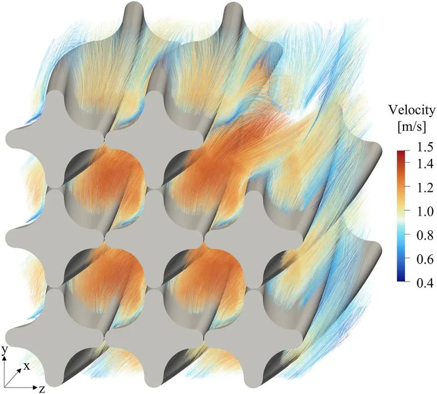
Transverse velocity is only about 4% of the axial value. Small as that sounds, it is what carries heat and mass into the neighbouring cells. Split one pitch into five cross-sections and you can see the core vortex, the one enclosed by four rods, drifting counterclockwise rather than sitting at the centre.
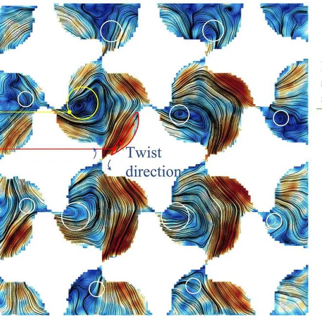
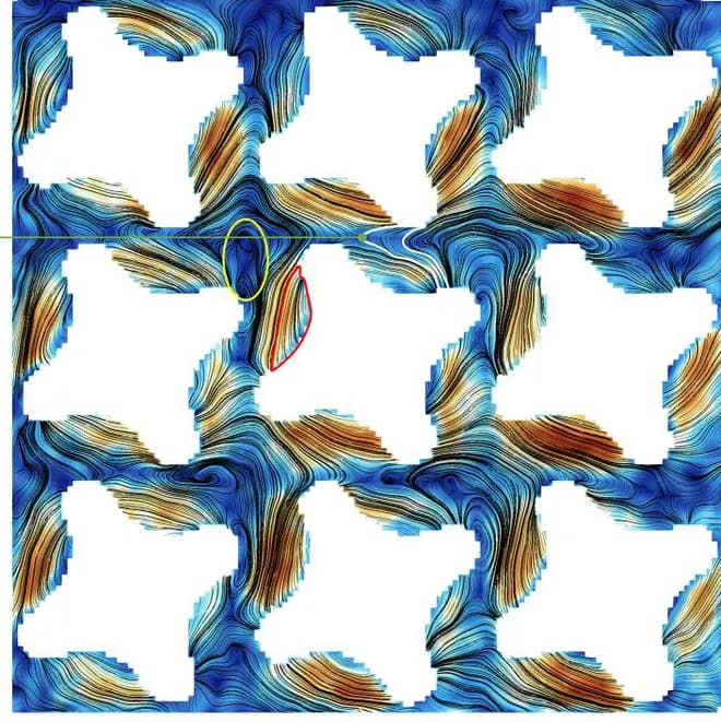
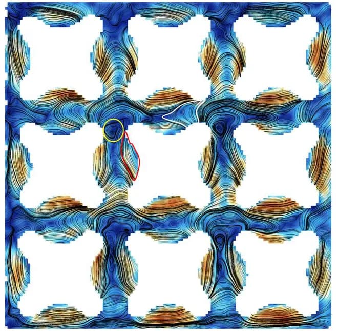
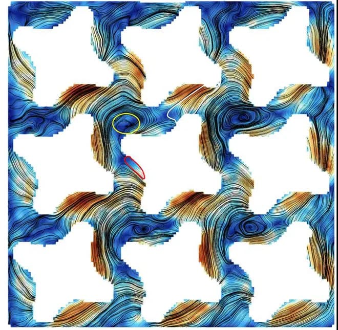
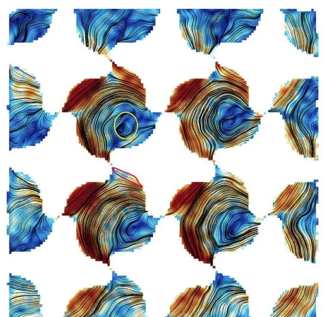

- Yellow circle — inner-core vortex
- Red outline — inter-subchannel shear layer
Axial position x/λ = 0.088
Here the rods have just begun to twist while still supporting one another. A sweeping motion wraps around each rod, and a coherent vortex already sits at the centre of the four surrounding rods.
Secondary-flow intensity
4.87%
of the axial velocity
Measured range 3.66 – 4.87% · Curve redrawn from Fig. 8 of the paper
Why does it drift
As the vortex approaches a wall, its mirror image on the far side pushes it along the wall, with a strength that grows as the distance shrinks. Add the pressure difference between the leading and trailing faces of each petal, and the vortex's equilibrium position shifts steadily along the axis.
10 — Into the next cell
The horizontal gaps are busier
We computed the flow through each of the four interfaces between the interior cells separately. As the core vortex rotates from the twelve o'clock toward the nine o'clock position, fluid is carried faster through the interfaces in that direction.
The two vertical interfaces collapse onto a similar trend regardless of measurement location, while the two horizontal ones show markedly stronger exchange. The drifting vortex interacts more directly with the neighbouring cell across the horizontal gaps.
What is counted here is the diversion crossflow driven by the mean pressure difference. The turbulence-driven interchange component was not covered by this campaign and is left for follow-on work.
11 — Takeaways
What this gives us
Secondary-flow intensity 3.66 – 4.87%
Mixing happens without grids
The pressure difference across each petal sustains the core vortex, and that vortex ferries fluid between cells. Mixing therefore occurs with no spacer grid, evidence that heat can be removed at a smaller pressure penalty.
There is now a reference to validate against
Velocity fields, uncertainty bounds, periodicity checks, and flow partitioning form one package, usable for calibrating subchannel correlations or validating CFD turbulence models.
What the experiment settles, and what it does not
Diversion crossflow from the mean pressure difference was computed directly from the measurements; the turbulence-driven interchange was kept separate. That separation makes clear, in verification and validation, which closures rest on experiment and which still rest on a model.
What remains
With a duct wall around a 3 × 3 array, the secondary-flow intensity is likely underestimated and the interior concentration overstated. Looking at wall-independent centre subchannels in a larger array comes next.
Source
H. Moon, H. Dong, S. Oh, M. Song, and S. Song, “In-depth flow investigation in subchannels of helical cruciform fuel using magnetic resonance velocimetry,” Physics of Fluids 38, 085111 (2026).
Measurement figures are from the paper above; the interactive elements and concept diagrams are redrawn from it.
This work was supported by the Innovative SMR Technology Development Agency (MSIT, No. RS-2024-00404240) and the National Research Foundation of Korea (MSIT, No. RS-2024-00461440).